Welcome to learning-curves’s documentation!
Learning-curves is Python module that extends sklearn’s learning curve feature. It will help you visualizing the learning curve of your models.
Learning curves give an opportunity to diagnose bias and variance in supervised learning models, but also to visualize how training set size influence the performance of the models (more informations here).
Such plots help you answer the following questions:
Do I have enough data?
Can I train my model with less data without reducing accuracy?
Is my training/validation set biased?
What is the best model for my data?
What is the perfect training size for tuning parameters?
Learning-curves will also help you fitting the learning curve to extrapolate and find the saturation value of the curve.
Installation
$ pip install git+https://github.com/H4dr1en/learning-curves#egg=learning-curves
To create learning curve plots, first import the module with
import learning_curves as LC.
Getting started
To get started, you can start with the following code:
import learning_curves as LC
from sklearn.datasets import make_regression
from sklearn.linear_model import SGDRegressor

X, Y = make_regression(n_samples=int(1e4), n_features=50, n_informative=25, bias=-92, noise=100)
lc = LC.LearningCurve()
lc.get_lc(SGDRegressor(), X, Y)
Output:
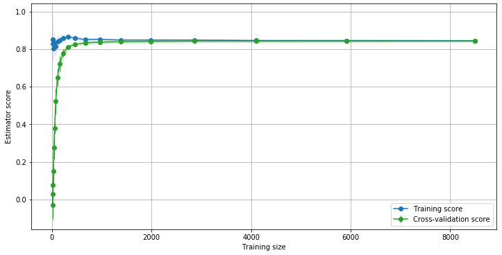
On this example the green curve suggests that adding more data to the training set is not likely to improve the model accuracy. The green curve also shows a saturation near 0.84. We can easily fit a function to any curve:
lc.plot(predictor="best")
Output:
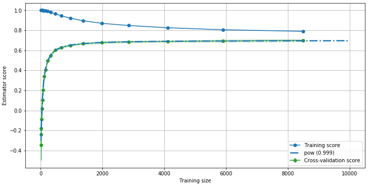
Here we used a predefined function, pow, to fit the green curve. The
R2 score is very close to 1, meaning that the fit is optimal. We can
therefore use this curve to extrapolate the evolution of the accuracy
with the training set size.
This also tells us how many data we should use to train our model to maximize performances and accuracy: near 2000, we achieved 99% of the maximal accuracy we can get for this model.
Custom Predictors
Predictors are object wrapping the fitting of learning curves.
You can create a Predictor like this:
predictor = Predictor("myPredictor", lambda x,a,b : a*x + b, [1,0])
Here we created a Predictor called “myPredictor” with the function
y(x) = a*x + b. Because internally SciPy optimize.curve_fit is
called, a first guess of the parameters a and b are required.
Here we gave them respective value 1 and 0. You can then add the
Predictor to the LearningCurve object in two different ways:
Pass the
Predictorto theLearningCurveconstructor:
lc = LearningCurve([predictor])
Register the
Predictorinside the predictors of theLearningCurveobject:
lc.predictors.append(predictor)
By default, 5 Predictors are instantiated:
defaults_predictors = [
        Predictor("pow",
                  lambda x, a, b, c, d: a - 1 / ( x/b - d)**c,
                  [1, 1, 1, 1],
                  lambda x, a, b, c, d: b * ( 1 / (a-x)**(1/c) + d)
                ),
        Predictor("inv",
                  lambda x, a, b, d: a / (1 + b/(x-d)),
                  [1, 1, 1],
                  lambda x, a, b, d: b / (a/x - 1) + d
                ),
        Predictor("inv_log",
                  lambda x, a, b, c, d: a - b/np.log(x-d)**c,
                  [1, 1, 1, 1],
                  lambda x, a, b, c, d: np.exp((b / (a-x))**(1/c) ) + d
                ),
        Predictor("pow_log",
                  lambda x, a, b, c, d, m, n: a - 1 / (x/b - d)**c + m*np.log(x**n),
                  [1, 1, 1, 1, 1e-2, 1e-2],
                  diverging=True,
                  bounds=([-np.inf, 0, 0, 0, 0, 0], [np.inf, np.inf, np.inf, np.inf, np.inf, np.inf])
              ),
        Predictor("inv_2",
                  lambda x, a, b, d, e: a / (e + b/(x-d)),
                  [1, 1, 1, 1],
                  lambda x, a, b, d, e: b / (a/x - e) + d
                )
    ]
Some predictors perform better (R2 score is closer to 1) than others, depending on the dataset, the model and the value to be preditected.
Find the best Predictor
To find the Predictor that will fit best your learning curve, we can
call get_predictor function:
lc.get_predictor("best")
Output:
(pow [params:[ 0.9588563 11.74747659 -0.36232639 -236.46115903]][score:0.9997458683912492])
Plot the Predictors
You can plot any Predictors fitted function with the plot
function:
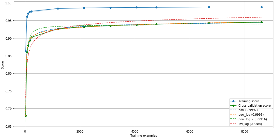
lc.plot(predictor="all")
Output:
Predictor bounds
Each parameter of a Predictor can be enforced to have values inside a
fixed interval using bounds:
lc.predictors[0].bounds
Output:
([-np.inf, 1e-10, -np.inf, -np.inf], [1, np.inf, 0, 1])
For example, the first parameter (the saturation parameter) is enforced to have values between [-inf, 1], because a R2 score cannot be > 1.
Average learning curves for better extrapolation
Multiple learning curves can be averaged to get a more accurate extrapolation, as well as a estimation of the error (standard deviation of the curve). This can easily be done using LearningCurveCombined class:
from sklearn.datasets import make_regression
from learning_curves import *
from xgboost import XGBRegressor

X, Y = make_regression(500, noise=0.5, bias=0.2, n_informative=50)
model = XGBRegressor(tree_method="hist")
lc = LearningCurveCombined(10)
lc.train(model, X, Y, n_splits=10, test_size=.2)
lc.plot(target=2000, figsize=(8,4))
Output:
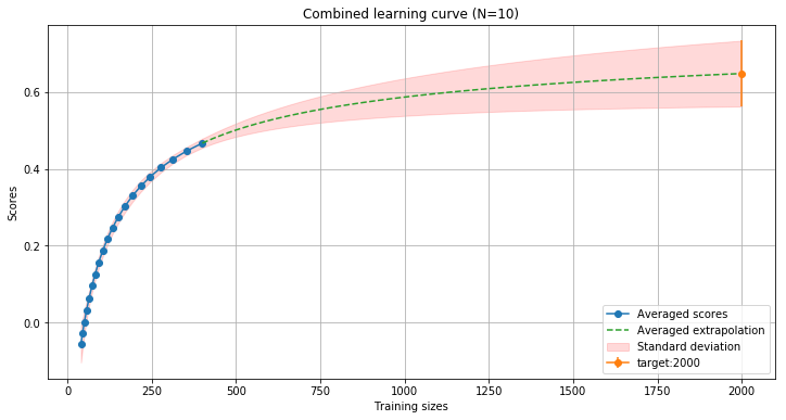
In this example, the LearningCurveCombined class computes 10 different learning curves and save them internally. Then the extrapolation is calculated by averaging each predictor results. To get the score of a particular training size, use the target() method:
lc.target(5000000)
Output:
(array([0.80658311]), array([0.27924702]))
This will give you the averaged scoore (0.8) and the standard deviation (0.279).
We can verifiy this by plotting the actual 10 learning curves computed:
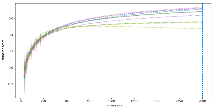
lc.plot_all(figsize=(12,6), what="valid", std=False, alpha=.1, alpha_fit=.5, target=2000, predictor="best", legend=False)
Output:
Evaluate extrapolation using mse validation
The goodness a fit is calculated using the R2 score. Another metric can be used: the mean-squared-error (or root-mean-squared-error). This can be done by excluding points from the fitting of the curve and using them for validation:
import learning_curves as LC
from sklearn.datasets import make_regression
from sklearn.linear_model import SGDRegressor

X, Y = make_regression(n_samples=int(1e4), n_features=50, n_informative=25, bias=-92, noise=100)
lc = LC.LearningCurve()
lc.get_lc(SGDRegressor(), X, Y, predictor="best", validation=0.2)
Output:
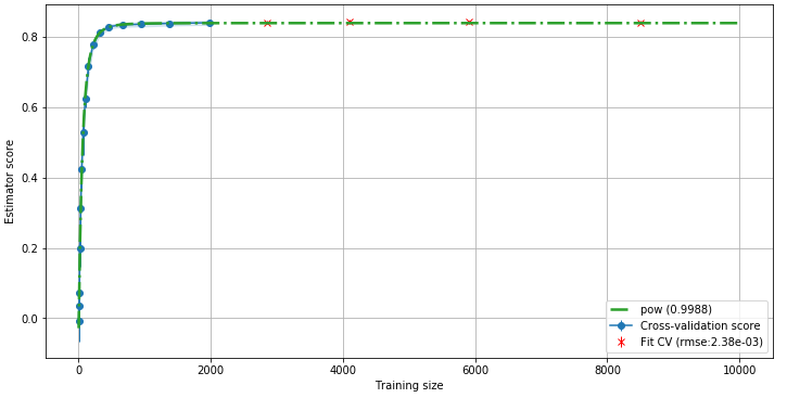
In this plot we can see that 20% of the points have been excluded from the fitting and have been used for calculating a RMSE (here, 2,38e-3). This RMSE is another indicator that we can safely extrapolate this curve and predict the score of the model trained with more data.
Compare Learning curves of various models
If you have multiple models, you can plot their learning curves on the same plot:
import learning_curves as LC
from sklearn.datasets import make_regression
from sklearn.linear_model import SGDRegressor
from sklearn.svm import SVR
from sklearn.neighbors import KNeighborsRegressor
from sklearn.ensemble import RandomForestRegressor
models = []
models.append(("SGDRegressor",SGDRegressor()))
models.append(("KNeighborsRegressor",KNeighborsRegressor()))
models.append(("SVR",SVR()))
models.append(("RandomForestRegressor",RandomForestRegressor()))
X, Y = make_regression(n_samples=int(1e4), n_features=50, n_informative=25, bias=-92, noise=100)
lcs = []
for name, model in models:
lc = LC.LearningCurve(name=name)
lc.train(model, X, Y)
lcs.append(lc)
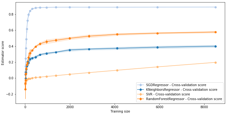
LC.LearningCurve.compare(lcs, what="valid")
Output:
Save and load LearningCurve instances
Because Predictor contains lambda functions, you can not simply save
a LearningCurve instance. One possibility is to only save the data
points of the curve inside lc.recorder["data"] and retrieve then
later on. But then the custom predictors are not saved. Therefore it is
recommended to use the save and load methods:
lc.save("path/to/save.pkl")
lc = LC.LearningCurve.load("path/to/save.pkl")
This internally uses the dill library to save the LearningCurve
instance with all the Predictors.
Find the best training set size
learning-curves will help you finding the best training set size by
extrapolation of the best fitted curve:
lc.plot(predictor="all", saturation="best", target=31668)
Output:
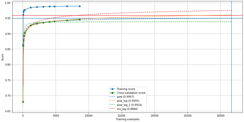
The horizontal red line shows the saturation of the curve. The
vertical blue lines shows the best accuracy we can get,
given a certain threshold (see below). We can use target
parameter to extrapolate the curves.
To retrieve the value of the best training set size:
lc.threshold(predictor="best", saturation="best")
Output:
(0.9589, 31668, 0.9493)
This tells us that the saturation value (the maximum accuracy we can get
from this model without changing any other parameter) is 0.9589.
This value corresponds to an infinite number of samples in our training
set! But with a threshold of 0.99 (this parameter can be changed
with threshold=x), we can have an accuracy 0.9493 if our
training set contains 31668 samples.
Note: The saturation value is always the second parameter of the
function. Therefore, if you create your own Predictor, place the
saturation factor in second position (called a in the predefined
Predictors). If the function of your custom Predictor is
diverging, then no saturation value can be retrieven. In that case, pass
diverging=True to the constructor of the Predictor. The
saturation value will then be calculated considering the max_scaling
parameter of the threshold_cust function (see documentation for
details). You should set this parameter to the maximum number of sample
you can add to your training set.
Compare the models performances
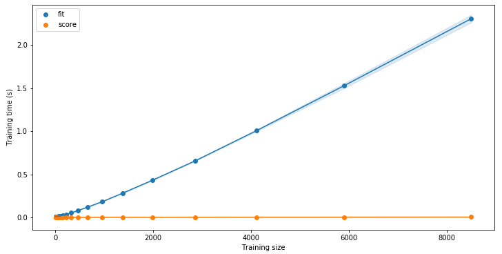
learning-curves also keeps track of the time elapsed during the
computation of the learning curves:
from sklearn.datasets import make_regression
from sklearn.ensemble import RandomForestRegressor

X, Y = make_regression(n_samples=int(1e4), n_features=50, n_informative=25, bias=-92, noise=100)
estimator = RandomForestRegressor()

lc=LC.LearningCurve()
lc.train(estimator, X, Y)
lc.plot_time()
Output:
As for the learning curves, you can easily compare the performances
using the LearningCurve.compare_time() function:
from sklearn.linear_model import SGDRegressor
from sklearn.svm import SVR
from sklearn.neighbors import KNeighborsRegressor
from sklearn.ensemble import RandomForestRegressor

models = []
models.append(("SGDRegressor",SGDRegressor()))
models.append(("KNeighborsRegressor",KNeighborsRegressor()))
models.append(("SVR",SVR()))
models.append(("RandomForestRegressor",RandomForestRegressor()))

lcs = []
for name, model in progress_bar(models):
    lc=LC.LearningCurve(name=name)
    lc.train(model, X, Y, verbose=10)
    lcs.append(lc)

LC.LearningCurve.compare_time(lcs, what="fit")
Output:
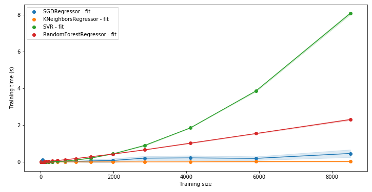
Having the times help you diagnose which model is likely to scale better with more data:
import matplotlib.pyplot as plt
fig, ax = plt.subplots(1,1, figsize=(12,6))

for lc in lcs:
    ax.plot(lc.recorder["fit_times_mean"], lc.recorder["test_scores_mean"])
    ax.scatter(lc.recorder["fit_times_mean"], lc.recorder["test_scores_mean"], label=lc.name)

ax.set_xlabel("Fit time (s)")
ax.set_ylabel("Accuracy (r2 score)")
ax.legend()
Output:
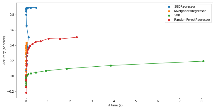
With this plot with see that KNeighborsRegressor, altough looking very promising and scalable in the previous plot, does not achieve to reach an accuracy such as SGDRegressor. SGDRegressor would probably be the best model for doing predictions on this dataset.